Navier-Stokes equation
We consider the incompressible Navier-Stokes equation in a domain ,
with velocity , pressure , density , dynamic viscosity , symmetric rate-of-strain tensor , and external volume force , w.r.t. to boundary conditions on . For an overview, see also Wikipedia.
Discretization
Weak formulation
In a weak variational formulation, we try to find and , such that
for , given .
The pair is thus in the product space where is also a product of spaces, i.e., . Later, this space will be approximated with a Taylor-Hood space of piecewise quadratic and linear functions.
Time-discretization
A linearized time-discretization with a semi-implicit backward Euler scheme then reads:
For find , s.t.
with , timestep , and given initial velocity .
Finite-Element formulation
Let be partitioned into quasi-uniform elements by a conforming triangulation . The functions and are approximated by functions from the discrete functionspace with and , where is the space of polynomials of order at most . The space will be denoted as Taylor-Hood space.
Let Grid grid be the Dune grid type representing the triangulation of the domain , then
the basis of the Taylor-Hood space can be written as a composition of Lagrange bases:
using namespace Dune::Functions::BasisFactory;
auto basis = composite(
      power<Grid::dimensionworld>(
        lagrange<2>(), flatInterleaved()),
      lagrange<1>(), flatLexicographic());
composite(...) to combine the different types for velocity and pressure space, while we
can use power<d>(...) for the d velocity component spaces of the same type.
For efficiency, we use flat indexing strategies flatInterleaved and flatLexicographic
to build a global continuous numbering of the basis functions.
See the tutorial Grids and Discrete Functions for more details.
Implementation
We split the implementation into three parts, 1. the time derivative, 2. the stokes
operator and 3. any external forces. For addressing the different components of
the Taylor-Hood basis, we introduce the treepaths _v = Dune::Indices::_0 and
_p = Dune::Indices::_1 for velocity and pressure, respectively.
Problem framework
We have an in-stationary problem consisting of a sequence of stationary equations
for each timestep, thus we combine a ProblemInstat
with a ProblemStat .
using namespace AMDiS;
ProblemStat prob{"stokes", grid, basis};
prob.initialize(INIT_ALL);

ProblemInstat probInstat{"stokes", prob};
probInstat.initialize(INIT_UH_OLD);
Time derivative
For simplicity of this example, we use a backward Euler time stepping and a linearization of the nonlinear advection term:
// define a constant fluid density
double density = 1.0;
Parameters::get("stokes->density", density);

// a reference to 1/tau
auto invTau = probInstat.invTau();

// <1/tau * u, v>
auto opTime = makeOperator(tag::testvec_trialvec{},
  density * invTau);
prob.addMatrixOperator(opTime, _v, _v);

// <1/tau * u^old, v>
auto opTimeOld = makeOperator(tag::testvec{},
  density * invTau * probInstat.oldSolution(_v));
prob.addVectorOperator(opTimeOld, _v);

for (int i = 0; i < Grid::dimensionworld; ++i) {
  // <(u^old * nabla)u_i, v_i>
  auto opNonlin = makeOperator(tag::test_gradtrial{},
    density * prob.solution(_v));
  prob.addMatrixOperator(opNonlin, treepath(_v,i), treepath(_v,i));
}
Stokes operator
The stokes part of the Navier-Stokes equation is a common pattern that emerges in several fluid equations.
for and .
// define a constant fluid viscosity
double viscosity = 1.0;
Parameters::get("stokes->viscosity", viscosity);

for (int i = 0; i < Grid::dimensionworld; ++i) {
  // <viscosity*grad(u_i), grad(v_i)>
  auto opL = makeOperator(tag::gradtest_gradtrial{}, viscosity);
  prob.addMatrixOperator(opL, treepath(_v,i), treepath(_v,i));
}

// <d_i(v_i), p>
auto opP = makeOperator(tag::divtestvec_trial{}, 1.0);
prob.addMatrixOperator(opP, _v, _p);

// <q, d_i(u_i)>
auto opDiv = makeOperator(tag::test_divtrialvec{}, 1.0);
prob.addMatrixOperator(opDiv, _p, _v);
External volume force
The force may be implemented as a vector-valued function of the global coordinates or any other expression that leads to a local force vector at the quadrature points, e.g.
using WorldVector = typename Grid::template Codim<0>::Geometry::GlobalCoordinate;
auto opForce = makeOperator(tag::testvec{},
  [](WorldVector const& x) { return WorldVector{1.0, 0.0}; });
prob.addVectorOperator(opForce, _v);
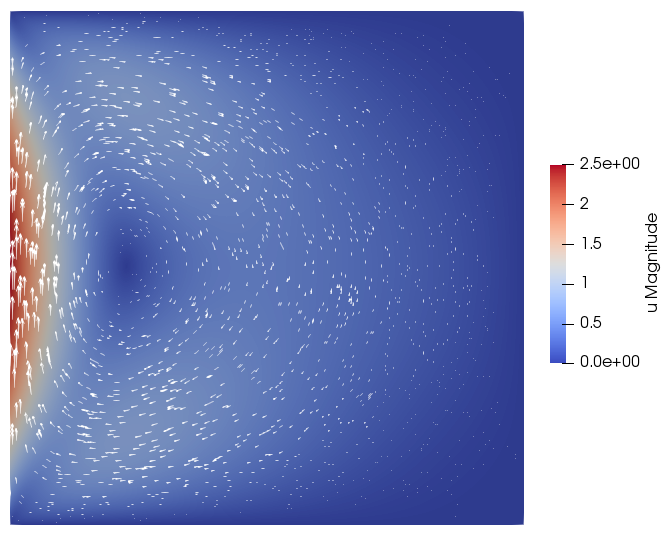
Numerical example
We consider a lid-driven cavity problem in a square domain with no external force, and with Dirichlet boundary conditions
Thus, the boundary value is zero on top, right, and bottom boundary and parabolic on the left boundary. The boundary condition is implemented, by first setting boundary ids for parts of the grid boundary and second, setting the Dirichlet value:
double vel = 1.0;
Parameters::get("stokes->boundary velocity", v1);

// define boundary values
auto g = [vel](WorldVector const& x)
{
  return WorldVector{0.0, v1*x[1]*(1.0 - x[1])*(1.0 - x[0])};
};

// set boundary conditions for velocity
prob.boundaryManager()->setBoxBoundary({1,1,1,1});
prob.addDirichletBC(1, _v, _v, g);
Simulation
The time-stepping process with a stationary problem in each iteration can be started
using an AdaptInstationary manager class:
// set initial conditions
prob.solution(_v).interpolate(g);

// start simulation
AdaptInfo adaptInfo("adapt");
AdaptInstationary adapt("adapt", prob, adaptInfo, probInstat, adaptInfo);
adapt.adapt();
Complete Example
The full source code of the Navier-Stokes example can be found in the repository at examples/navier_stokes.cc.
Compile with
cmake --build build --target navier_stokes.2d
and run with
./build-cmake/examples/navier_stokes.2d examples/init/navier_stokes.dat.2d
The flow field with density=1, viscosity=1 and boundary velocity=10 will look like